
Cell Reports · Track 1 · Tutorial 9 of 12
Sort, filter and chart a Cell Report
Available on ProPremium
Readers can sort, filter and freeze a Cell Report in View to read it their way, without changing the report. Charts are the other way round: you add them in the editor, anchored to a cell, and they read the consolidation each time the report is opened, like the cells do.
1Sort in View
- Open the report in View, and click a cell in the table you want to sort, such as D4.
- Under View in the toolbar, open Sort and filter, and click Sort Z to A.
BrizoConsol finds the table around the cell you clicked — the block of filled cells up to the first empty row and column, as a spreadsheet does — and sorts its rows by the clicked column. For more control, click Custom Sort…: choose Sort by a column, the Order, and whether My data has headers, then click Sort.
Rows keep their own values; only their order changes. Nothing is recalculated and nothing is saved. Clear Sort puts the rows back.
2Filter and freeze in View
- Click a cell in the table, open Sort and filter, and click Filter with the table’s range.
- Click the filter button on a heading. Search the values, untick the ones to hide — or use (Select all) — and apply.
- From Freeze Panes, choose Freeze Top Row, Freeze First Column, or Freeze Panes at the selected cell.
The filter menu on a heading also sorts by that column. Clear Filter shows every row again; Remove Filter takes the filter buttons off. Clear view drops the sort, filter and freeze together.
These are the reader’s own: the next person to open the report sees it as saved. To make a freeze part of the report, set it in the editor.
3Insert a chart
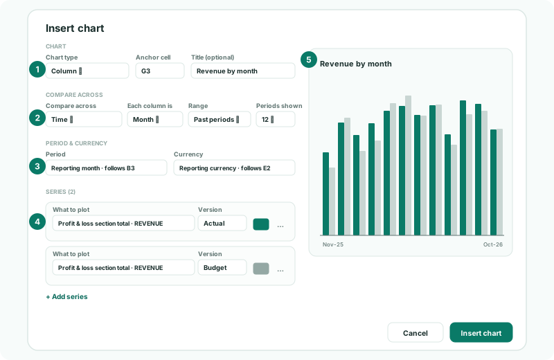
- In the editor, click G3, then Insert chart under Insert in the toolbar.
- Under Chart, choose Chart type Column, keep Anchor cell G3, and enter the Title Revenue by month.
| Chart type | Use it for |
|---|---|
| Column, Line, Area | A figure over time. |
| Bar | Comparing items or entities, when their names are long. |
| Pie, Doughnut | Shares of a whole at one point, such as revenue by entity. |
4Choose what to compare and plot
- Under Compare across, choose Time. Set Each column is Month, Range Past periods, and Periods shown 12.
- Under Period & currency, keep Period on Reporting month and Currency on Reporting currency. With the choices from Let readers choose the entity, period and currency on the sheet, they follow B3 and E2.
- Under Series, click + Add series. In What to plot, choose Profit & loss section total, then REVENUE, and keep Version Actual.
- Click + Add series again for the budget: the same section with Version Budget, and a different Colour.
- Check the preview, and click Insert chart.
| Compare across | Each bar or point is |
|---|---|
| Time | A month, quarter, half year or year, going back (Past periods), forward (Upcoming periods), or across This fiscal year. |
| Accounts, sections or lines | One of the items you pick in Which items to compare. |
| Entities | One of the companies you pick in Which entities to compare. |
Under Display, set the Width and Height in pixels, and whether to show the legend and Value labels.
5Change or delete a chart
Click the chart in the editor to open it again, change it, and click Save changes; Delete chart removes it. Changes apply to that chart only.
Check
Save and View the report. The chart shows 12 columns ending in October 2026, the last one matching B4’s revenue, with the budget beside each. Choose Sep-2026 in B3: the chart’s last column becomes September.
6If something goes wrong
| What you see | What to do |
|---|---|
| Sort sorts the wrong rows | The table around the clicked cell runs to the first empty row and column. Use Custom Sort… and check the range it names. |
| The sort included the headings | Tick My data has headers in Custom Sort…. |
| The chart is empty | A series has nothing to plot, or the version has no figures for the months shown. Check What to plot and Version. |
| The chart doesn’t follow the month chosen in B3 | Its Period is a Fixed month. Choose Reporting month, or Link to a cell. |
| The chart covers the figures | Move its Anchor cell to the right of the table, or reduce its width. |
Want more detail? See the documentation