
Cell Reports · Track 1 · Tutorial 4 of 12
Write formulas and use the formula helper
Available on ProPremium
Bound cells bring the figures in; formula cells work with them. A Cell Report’s formulas are spreadsheet formulas, calculated each time the report is opened, so a variance or a margin is always worked out from this month’s figures.
1Know what a formula cell is
Anything you type that starts with = is a formula, and the cell’s Cell type becomes Formula by itself. The formula is kept in the cell; the result is worked out by the report engine each time the report is opened, with the same functions and rules as Excel.
| Operators | + − * / and ^, with brackets; & joins text; =, <, >, <=, >= and <> compare. |
|---|---|
| References | A cell, such as B4, or a range, such as B4:B6. |
| Functions | The functions in the formula helper: Maths, Statistics, Logic, Lookup, Text and Date. See step 5. |
A formula can read any cell, whatever its type: bound figures, typed numbers and other formulas.
2Write the variance by clicking
- Click D4, and type = in the formula bar, beside fx.
- Click B4. While the formula starts with =, clicking a cell drops its reference in: the bar reads =B4.
- Type -, click C4, and press Enter.
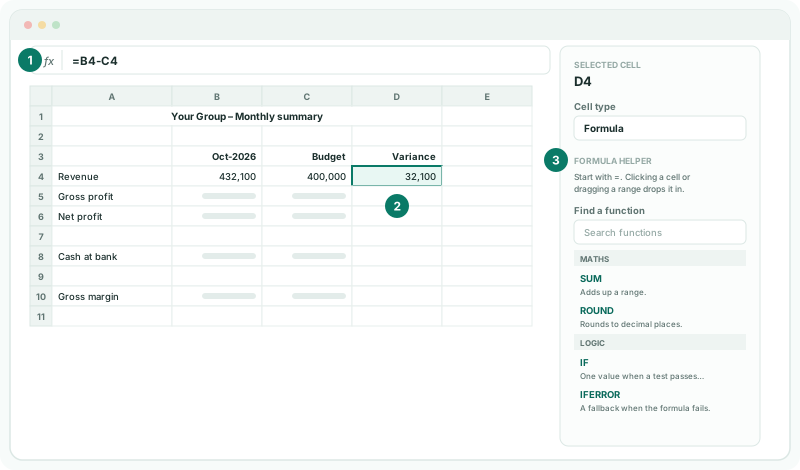
Instead of clicking, you can move the reference with the arrow keys while you write, or drag across cells to put in a range. Enter confirms the formula; Escape leaves it unchanged.
D4 shows the result straight away. If October’s budget revenue is, say, 400,000, D4 shows 32,100: 432,100 − 400,000.
3Fill the formula down
- Select D4.
- Drag the small square at the corner of the selection — Drag to fill — down to D6.
Each copy moves its references with it: D5 reads =B5-C5 and D6 =B6-C6. Copying and pasting a formula moves its references the same way. One formula written well serves the whole column.
4Fix a reference with $
Add a gross margin row: in A10 type Gross margin. Then:
- Click B10 and type =B5/B$4.
- Drag B10’s fill square across to C10.
- Select B10 to C10 and set Number format to Percentage.
C10 reads =C5/C$4: the column moved, but the row 4 stayed, because of the $ in front of it. A $ fixes what follows it: $B4 fixes the column, B$4 the row, and $B$4 both. Use it whenever a filled formula must keep pointing at one cell, such as a total or a rate.
5Find a function with the formula helper
Add the variance as a percentage. A variance % divides by the budget, and a month with no budget would divide by zero, so guard it.
- In E3 type Variance %. Click E4 and type =.
- Under Formula helper in the inspector, type error in Find a function, and click IFERROR. It goes into the formula bar as IFERROR(, and the helper shows what it does and an example.
- Complete the formula: =IFERROR(D4/C4,0), and press Enter.
- Fill E4 down to E6, and set E4 to E6 to Percentage.
With the search empty, the helper lists the functions by group. Hover over a function to see its example.
| Group | Functions |
|---|---|
| Maths | SUM, ROUND, ABS, MIN, MAX, SUMPRODUCT, POWER, SQRT, MOD, INT |
| Statistics | AVERAGE, COUNT, COUNTA, MEDIAN, STDEV, LARGE, SMALL |
| Logic | IF, IFERROR, AND, OR, NOT |
| Lookup | SUMIF, COUNTIF, INDEX, MATCH, VLOOKUP, RANK |
| Text | TEXT, CONCATENATE, LEFT, RIGHT, MID, LEN, TRIM, VALUE |
| Date | DATE, YEAR, MONTH, DAY, EDATE, EOMONTH, TODAY |
6Check and save
- Click Save, then View.
Check
D4 to D6 equal the actual less the budget in each row, E4 to E6 show the variance as a percentage of the budget, and B10 and C10 show gross profit as a percentage of revenue. Open the report for another month: every result follows the new figures without any change to the formulas.
7If something goes wrong
| What you see | What to do |
|---|---|
| The formula shows as text | It doesn’t start with =. Retype it with = first. |
| #DIV/0! | The formula divides by an empty or zero cell. Wrap it in IFERROR, as in step 5. |
| #NAME? | A function name is misspelled, or text is missing its quotes. Pick the function from the formula helper. |
| #REF! | A row or column the formula read was deleted. Correct the reference. |
| A filled formula points at the wrong row | The reference that should stay fixed has no $. Add it, as in step 4, and fill again. |
| Clicking a cell moves the selection instead of adding a reference | The formula bar doesn’t start with =. Type = first. |
Want more detail? See the documentation