
Cell Reports · Track 1 · Tutorial 8 of 12
Format and highlight with conditional formatting
Available on ProPremium
A reader should see at a glance which variances need attention. Conditional formatting colours a cell by its value each time the report is opened, so the highlight follows the figures: a variance that turns negative next month turns red next month.
1Know the conditions
| Condition | Highlights |
|---|---|
| Greater than, Less than, Equal to | Cells whose value compares to the Comparison value. |
| Between | Cells from the Comparison value up to the Upper value, both included. |
| Text contains | Cells containing the Text to find, in any case. |
| Largest absolute differences | The given Number of cells furthest from zero, either way, with one colour for positives and one for negatives. |
| Largest deteriorations | The given Number of cells with the lowest values. |
Rules belong to the sheet. Each has a Cell range, a condition and a Fill color and Text color. They apply to bound figures and formula results alike, and they are kept when the report is exported to Excel.
2Colour the variances
- In the editor, select D4 to D6, and click Conditional formatting under Styles in the toolbar. The Cell range is filled in with D4:D6.
- Choose Less than, enter 0 as the Comparison value, and pick a light red Fill color and a dark red Text color.
- Click Add Rule.
- Set Cell range to D4:D6 again, choose Greater than and 0, pick a light green fill and a dark green text, and click Add Rule.
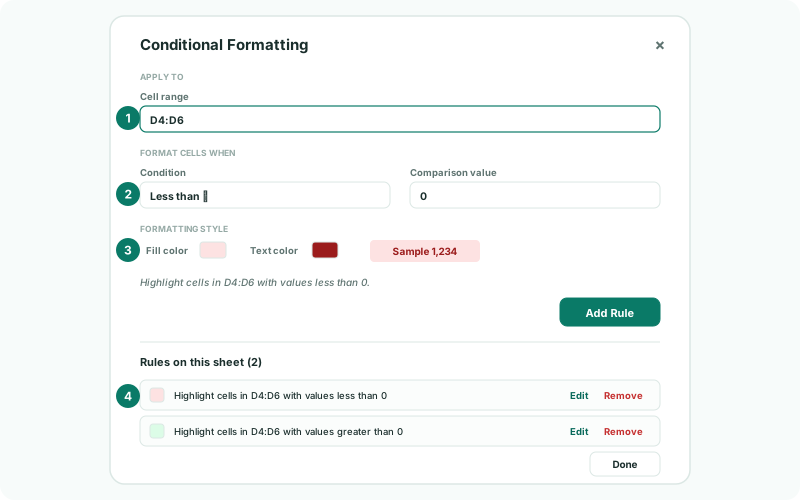
Under the colours, the dialog reads the rule back as a sentence, such as Highlight cells in D4:D6 with values less than 0, so you can check it before you add it. The sample shows the colours on a figure.
Do the same for E4:E6, the variance %. A revenue or profit variance below zero is unfavourable; for a cost line, where a positive variance is the bad one, swap the colours on that row’s range.
3Pick out the largest variance
- Set Cell range to D4:D6, choose Largest absolute differences, and enter 1 as the Number of cells.
- Under Positive values pick a strong green fill with white text, and under Negative values a strong red fill with white text.
- Click Add Rule, then Done.
The variance furthest from zero now stands out, in green if it is above budget and red if it is below. When two rules match the same cell, the one lower in the list sets the colours, so keep the stronger highlight last.
4Change or remove a rule
Open Conditional formatting again. The list Rules on this sheet shows each rule with its colours. Click Edit to change one, then Save Changes, or Cancel Edit to leave it. Click Remove to delete one.
5Check it
- Click Save, then View. Choose another month in B3.
Check
Each variance below zero is red and each above zero green, and the largest one carries the strong colour. When the month changes, the colours move with the new figures. Export to Excel: the same rules are in the workbook.
6If something goes wrong
| What you see | What to do |
|---|---|
| Enter a valid range, such as B2:D5. | The Cell range isn’t a cell or a range. Enter it as a start and end cell, such as D4:D6. |
| A rule colours nothing | Check the range covers the cells, and the Comparison value is a number for Greater than, Less than, Equal to and Between. |
| A cell shows the wrong colour | Two rules match it, and the later one wins. Change the order by removing and adding the rule again. |
| The colours stop after inserting rows | Check the rule’s range still covers the cells you meant. Edit it if not. |
Want more detail? See the documentation